Psychoacoustics & Sound Quality - An Introduction

Psychoacoustics and Sound Quality Metrics

Most of the time, in acoustics and NVH, we are interested in the overall sound pressure level (OASPL) and the frequency content of acoustic events. This is useful as it gives us a simple basis for target setting and monitoring the status of development.

However, these metrics do not always tell us the whole story, as they do not reflect the subjective, perceived quality of the sound – rather it only gives an objective rating of the output sound pressure levels.

The assessment of ‘Sound Quality’ utilises a series of psychoacoustic parameters and metrics. These metrics attempt to give us further information about the sound source under investigation, rather than simply a measure of noise level. This information is invaluable to NVH engineers, as it allows us to tune automotive systems in ways which not only decrease the noise level, but also increased the perceived sensory pleasantness of a sound.

Of course, there is a limit to the accuracy of these metrics, as we are attempting to objectively quantify what is a very personal, subjective experience. Each individual listener will have his or her own preferred acoustic characteristics, but nevertheless psychoacoustic metrics give us insight into what is likely to be a preferred sound by the majority of listeners.

Within this blog post, we are going to look at the most commonly used sound quality metrics in NVH engineering and the wider acoustic engineering industry.

Loudness

Loudness is one of the cornerstones of sound quality. Not to be confused with sound pressure level (SPL), Loudness attempts to estimate the ‘perceived’ sound level experienced by a listener. In contrast to standard SPL measurements, Loudness takes into account the masking effects of the human auditory system and the influence of critical bands. The unit of Loudness is the Phon (and often also the Sone), developed by Barkhausen in the 1920’s. A Phon is equal in value to the decibel level of a plane wave, frontal incidence 1kHz tone. A Sone is the equivalent to a 40dB 1kHz tone. Equal loudness contour curves are used to assess the Loudness level at varying frequencies. Loudness can also be assessed over a frequency range, using Bark bands (or critical band rate) named after Barkhausen. Rather than using a typical frequency scale in Hz, Bark bands correspond to the critical bands of the human ear. When we assess Loudness versus Bark bands, we refer to this as Specific Loudness.

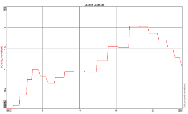
The critical bands (Bark bands) of the human ear are a key component to all sound quality metrics.

Sharpness:

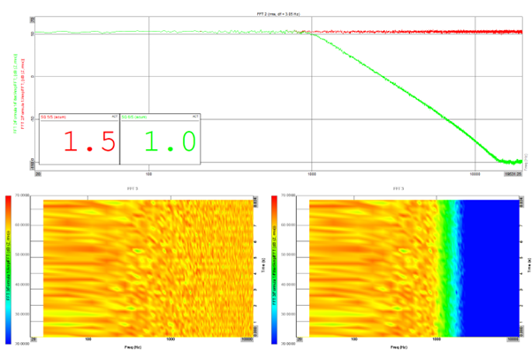
The Sharpness metric is used to define the spectral shape of the sound, with a particular bias towards high frequency sounds (which increase ‘brightness’) and the centre-frequencies of narrow-band sounds.

The unit of Sharpness is the Acum, which is equal to narrow-band noise (one critical band wide) at a centre frequency of 1kHz with a level of 60dB.

An example is shown below, where we have analysed a typical pink noise signal and a low pass filtered version. As expected, the raw noise signal (which contains more high frequency energy) produces a higher Sharpness level.

Based on subjective evaluations conducted by Fastl and Zwicker, it is generally the case that sensory pleasantness decreases with an increase in Sharpness.

In general, the overall level of the sound will have very little bearing on the Sharpness metric. However, the Aures model of Sharpness also considers the Loudness of the sound being analysed. This can be a useful model in some cases.

Roughness:

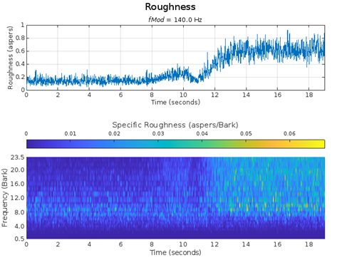
Roughness is an amplitude modulation (AM) metric. This means that is used to identify variations in Loudness over time which can lead to sensations of ‘roughness’ to the listener.

The most sensitive fluctuation frequency for the Roughness metric is around 70Hz. Individual amplitude fluctuations at this rate are not readily apparent to the listener due, which is what generates the ‘rough’ sensation of the sound. It is also noted that AM frequencies of 15Hz to 300Hz can generate the roughness sensation and contribute to the Roughness metric.

The unit of Roughness is the Asper, which is equal to a 60dB, 1kHz tone which is 100% modulated by a 70Hz modulator. As with the standard Sharpness model, the metric is not affected by the overall level of the sound, rather it is controlled by the modulation characteristics.

Generally, roughness can be generated by motor systems where there are relatively high fluctuations in Loudness due to meshing effects or system run-out.

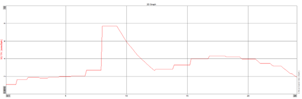
We can demonstrate the calculation of Roughness using a simple MaxMSP patch. This application is generating a broadband noise signal which is modulated by a 70Hz sine signal. The modulation depth can be controlled, and the output is increasingly modulated over time.

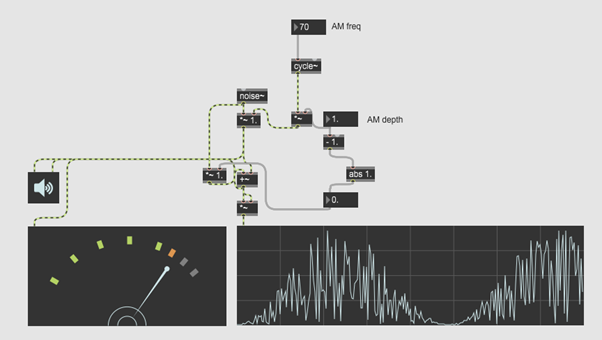
As you can see on the plot below, the Roughness increases as we introduce additional modulation depth to the signal.

As with Sharpness, sensory pleasantness tends to decrease with increasing roughness.

Fluctuation Strength:

Similarly to Roughness, Fluctuation Strength analyses frequency modulation characteristics of a signal. However, while the Roughness metric is most sensitive to AM at 70Hz, Fluctuation Strength has its sensitivity peak at 4Hz. Modulations in this frequency range are expected to be clearly audible to a listener.

There is a transition region at a modulation frequency of around 20Hz, where perceived fluctuation transforms to a sense of roughness. This is not a hard border, but more of a smooth crossover between the two sensations.

The unit of Fluctuation Strength is the Vacil, which is equal to a 60dB, 1kHz tone which is 100% modulated by a 4Hz modulator.

Using the previously discussed MaxMSP patch, we can demonstrate the analysis of Fluctuation Strength. The only difference this time is the modulator frequency, which is set at 4Hz.

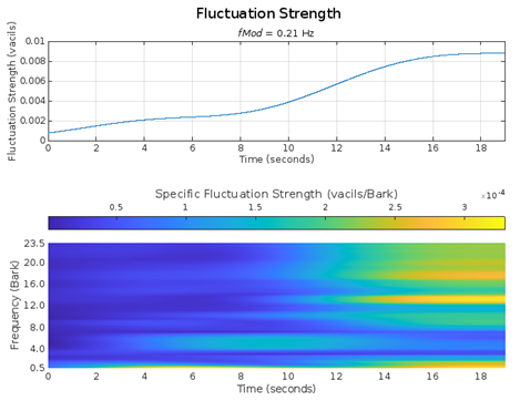
As you can see, the Vacil level increases as the modulation depth increases.

Prominence Ratio

The final metric we are going to look at is the Prominence Ratio. This is an analysis of tonality, but additionally, it tells us how prominent a tone is within the complete acoustic signal. It may be a case that a system is very tonal, however, NVH engineers also need to consider how prominent (or audible) that tone actually is to listeners to define if there is an issue which needs to be resolved.

The calculation of Prominence Ratio requires input from the Specific Loudness metric we discussed previously. As you can see from the plot shown in the Loudness section, the human hearing range is split in 24 bands (critical bands). The plot below shows an analysis of a 1kHz sine wave combined with a pink noise masking signal. This analysis is a specific loudness plot, showing loudness per Bark band.

You can clearly see the delineation between the critical bands along the x-axis of the plot.

The Prominence Ratio method calculates the overall SPL in the critical band containing the tone which is to be assessed, along with the overall SPL in the adjacent upper and lower critical bands.

Once these values are known, a delta value, between the upper, lower and middle critical bands can be calculated. For tones above 1kHz, the delta value must be above 9dB for the tone be classed as prominent.

There are other, similar methods available for assessing tonal prominence, such as tone-to-noise ratio and tone-in-band.

We hope that this blog post is useful. Obviously, it is a very short introduction to a very complex topic, and we hope to add more topics such as this to the blog over time. If you are interested in our Sound Quality analysis services, then please feel free to reach out.