FFT & Phase

FFT (Fast Fourier Transform) analysis is one of the key components of NVH analysis, and acoustic engineering as a whole.

The principal dates back to Carl Friedrich Gauss's work in 1805, which was later superseded by work conducted by Joseph Fourier in 1822. What Gauss and Fourier both proposed was that any signal (sound) can be generated using combinations of sine waves of varying frequency and phase relationships.

The inference being that the inverse is also true – any sound can be split into component frequency bands with corresponding phase values. This is the application of FFT which is most useful within NVH engineering. We can effectively capture an audio signal and transform this into the frequency domain with the use of FFT analysis.

To understand the basic process, there are a number of steps which need to be considered. Firstly, we need to have a basic understanding of quantization (the process of converting an analogue acoustic signal to a digitized signal which can be interpreted by a computer system).

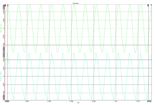
In order to do this, data acquisition systems ‘sample’ the continuously variable acoustic signal into discrete values at a specified rate (known as the sample rate). This is demonstrated in the plot below – the top trace shows the instantaneous pressure fluctuations (as would be received at a microphone diaphragm) while the lower trace shows the signal being sampled at discrete intervals.

One key point which must be considered when selecting the acquisition sample rate is defined by Nyquists Theorem. This states that ‘a sinusoidal function in time or distance can be regenerated with no loss of information as long as it is sampled at a frequency greater than or equal to twice per cycle.’ Or in simple terms, the sample rate must be at least twice the frequency component of interest.

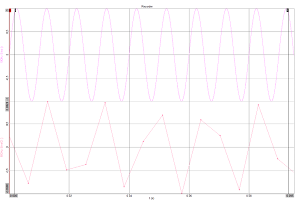
This is necessary as it allows two sample points to be present on each sine cycle, allowing the peaks and troughs to be accurately defined. If the sample rate is too low, then an effect knows as aliasing (in acoustics) or foldback (in audio engineering) occurs. This effectively ‘tricks’ the quantisation process into thinking that the input frequency is actually lower than in reality, and the alias frequency is then folded-back into the spectrum. An example is shown below, the top trace shows a correctly sampled 100Hz sine wave, whereas the lower trace shows the same signal sampled with a sample rate below the Nyquist frequency. As you can see, this will be interpreted by the analysis system as an approximately 50Hz signal.

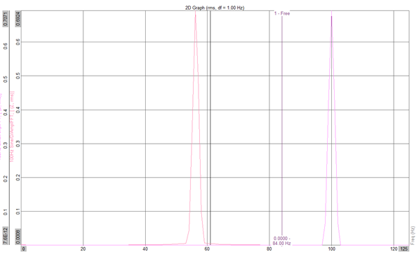
The subsequent frequency spectrum is shown below. As you can see, the low sample-rate signal is showing an inaccurate frequency of 60Hz.

Once the signal has been acquired, there are a few other FFT parameters which must be understood. The first is the frequency resolution and the frame size, these are intrinsically linked. The frequency resolution (defined in Hz) describes the width of the frequency bins of the FFT analysis. For example, a 1Hz resolution will split the signal into 1Hz wide bands (bins). FFT analysis allows us to view down to fractions of a Hz – however there is a trade-off…..

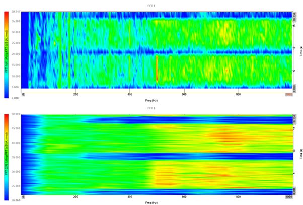
As the FFT analysis produces one frequency bin for each sample of the input data, a high frequency resolution will lead to a very low time resolution (as the sample rate will define how much time data is required to compute the requested frequency resolution). For example, assuming a signal sampled at 50kHz, and a requested resolution of 1Hz, 1 second of time data will be lumped into one block and analysed: If we request 0.1Hz resolution, the calculation will require 10 seconds of time data. The amount of time data required is known as the Frame Size (in seconds). There is always a trade-off between time and frequency resolution with FFT analysis.

The colourmaps below show the same signal analysed with 2 different frequency resolutions and frame sizes. The top plot has a fine frequency resolution, whereas the lower plot has a fine time resolution. You can clearly see how the inverse parameter is smeared across the analysis window.

Another important consideration is the windowing function, this transforms the input time data in order to shape it to a suitable input signal (preventing leakage). Many different windowing functions are available, the most common of which are the Hanning and Hamming windows. However there are specific windows for specific applications.

Another useful output of the FFT analysis (for NVH Engineering) is the phase response. In its simplest form, the phase response of a sine wave tells us where in the cycle the signal is at a specific time (usually displayed in degrees).

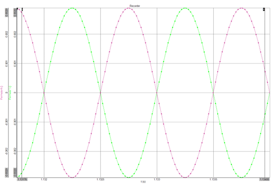
The plot below shows two sine waves which are 180° out-of-phase:

Analysis of phase can be incredibly useful to NVH engineers. It is used as an input to many advanced signal processing algorithms (such as coherence and coherent PSD), and it is also a key component of acoustic holography (acoustic cameras). It can also be used for balancing of rotating machinery and even defining damaged teeth in a gearset. In vibration and modal analysis, phase is used to highlight resonances, where a lag of 90° occurs between the input and output response of a dynamic system.

We hope that this basic introduction to FFT and Phase has been useful, and we welcome any feedback. If you feel that ARC can further assist you in your NVH or Acoustics projects – then please feel free to contact us.